Quickstart

This page walks you through a minimal, complete WAH-i workflow: from launching the app to obtaining an optimised microphone geometry and exporting results.

All versions of WAH-i (Windows, macOS, MATLAB) run the same optimiser core. Differences in confirmed appearance may arise due to font availability or screen resolution, but results are identical.

1) Launch WAH-i

Deployed app: open WAH-i from the Applications / Start menu.
MATLAB: run:
```
wahi_gui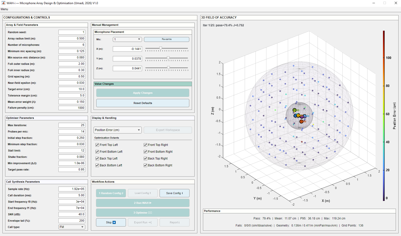
```
Installed App: Launching WAH-i on Windows / macOS. The app window is fixed-size to ensure a consistent layout across platforms.

Note

The deployed app window is intentionally non-resizable to maintain a consistent panel layout. Advanced users can customise layout behaviour when running from MATLAB.

2) Create or load a microphone geometry

You can start from scratch or reuse an existing configuration:

Random Config Generates a random geometry for the selected number of microphones.
Load Config Loads a previously saved geometry from CSV, automatically updating the display.

The Random Seed ensures reproducibility: using the same seed will generate the same random geometry and optimisation trajectory.

Randomised 4 microphone configuration example — Two example randomised microphone geometries generated using 4 and 6 microphone counts with the same random seeds. Randomisation provides diverse starting points for optimisation while remaining fully reproducible.

Randomised 6 microphone configuration example — Two example randomised microphone geometries generated using 4 and 6 microphone counts with the same random seeds. Randomisation provides diverse starting points for optimisation while remaining fully reproducible.

Tip

Loading a previously “good enough” configuration is an effective way to refine designs in stages and compare alternatives.

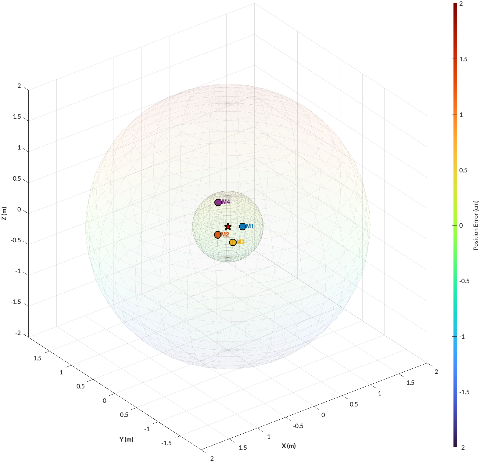
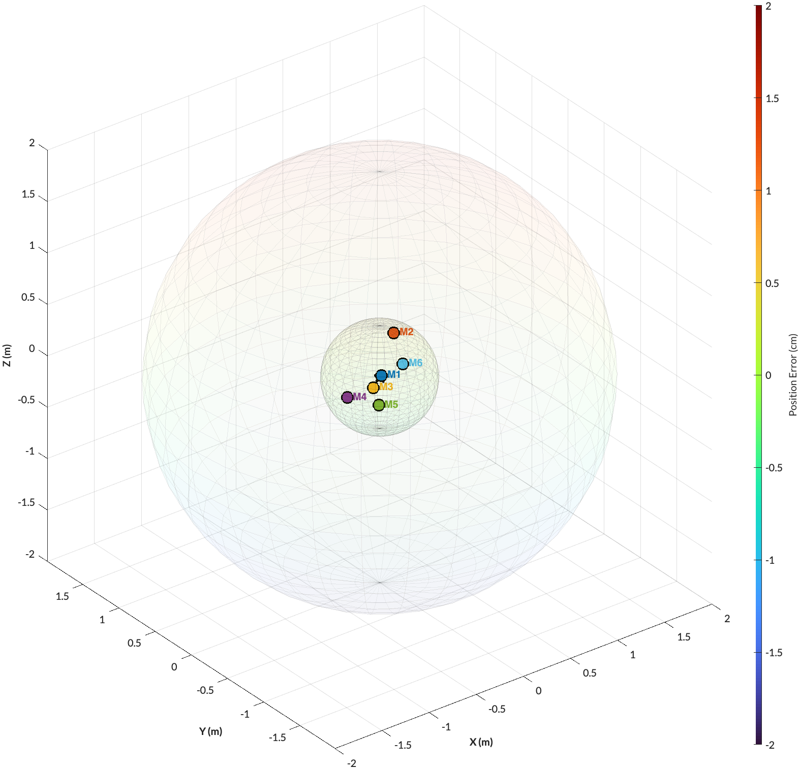
3) Define the Field of Accuracy (FoA)

The Field of Accuracy (FoA) specifies where in space localisation performance is evaluated and optimised. Rather than optimising uniformly over all directions and distances, WAH-i allows you to focus computational effort on the regions that matter most for your task.

In Array & Field Parameters, set:

FoA outer radius (R) and inner radius (Rin) to define the spatial shell of interest
Grid spacing, starting coarse for exploration and refining later for precision
Minimum source–microphone distance to avoid near-field degeneracies and unstable solutions

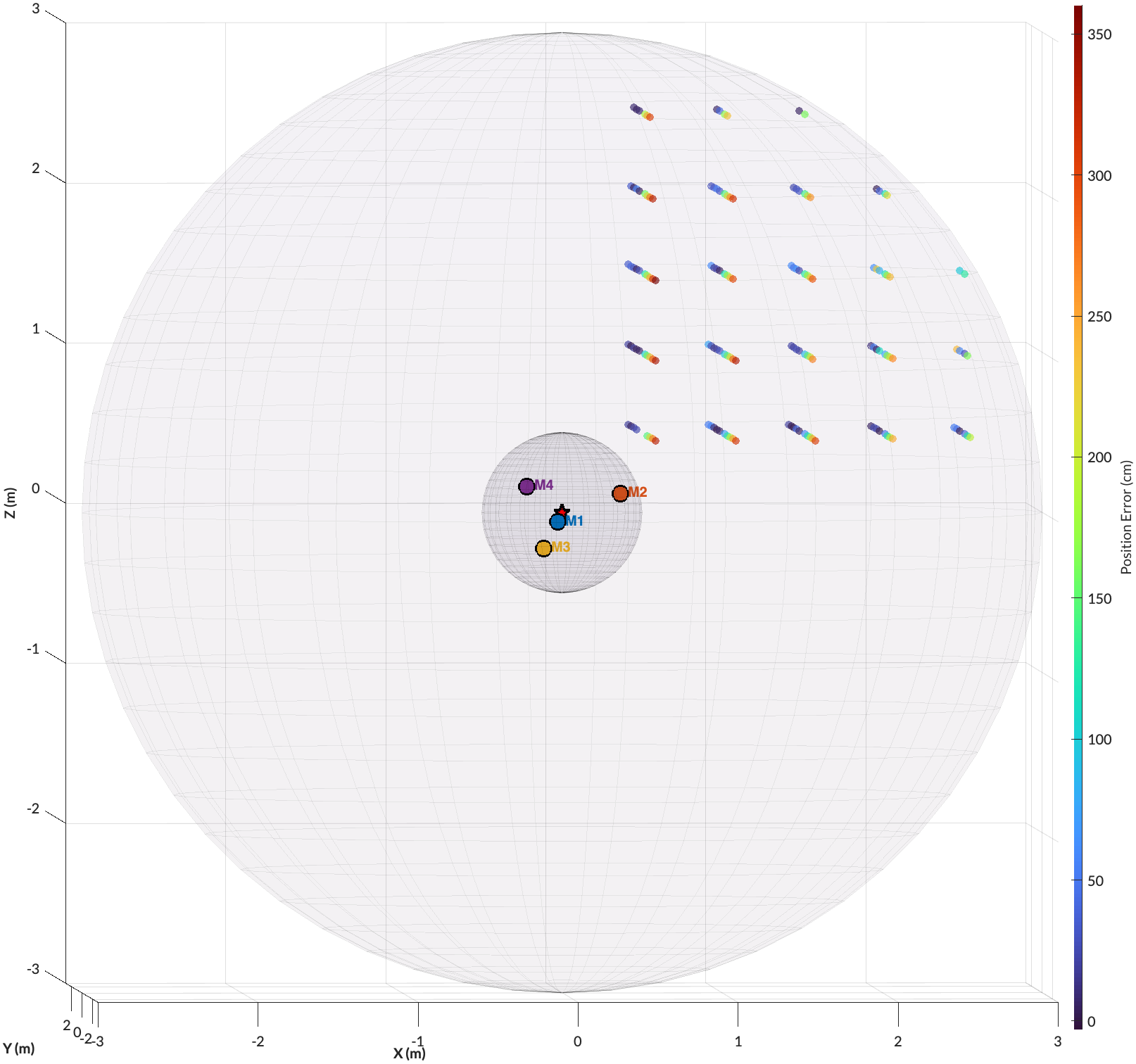
In addition, the octant selection checkboxes allow you to restrict optimisation to specific spatial sectors (e.g. front-facing, elevated, or lateral regions). Combined with tailored inner/outer radius ranges, this provides a powerful way to custom-define the spatial regions that matter for your experiment or deployment.

This is particularly useful when:

Targets are expected only in a known sector (e.g. forward flight, ground-facing arrays)
Certain regions are mechanically inaccessible or irrelevant
You want to trade global coverage for higher accuracy in a restricted volume

Once these parameters are set, click Apply Changes to commit the FoA definition before running or optimising.

Example FoA Configurations

Front-Top Field of Accuracy. FoA Outer R 3m, FoA Inner R Default. Unoptimised Run — Two example Fields of Accuracy. In the second example, the inner radius is increased to 2m, creating thinner shell of FoA. The selected octants are limited to the front-top regions. In both cases, the accuracy estimations are unoptimised (only Run WAH stage executed)

Front-Top Field of Accuracy. FoA Outer R 3m, FoA Inner R 2m. Unoptimised Run. — Two example Fields of Accuracy. In the second example, the inner radius is increased to 2m, creating thinner shell of FoA. The selected octants are limited to the front-top regions. In both cases, the accuracy estimations are unoptimised (only Run WAH stage executed)

Important

Any change to geometry or field parameters requires clicking Apply Changes before running evaluation or optimisation.

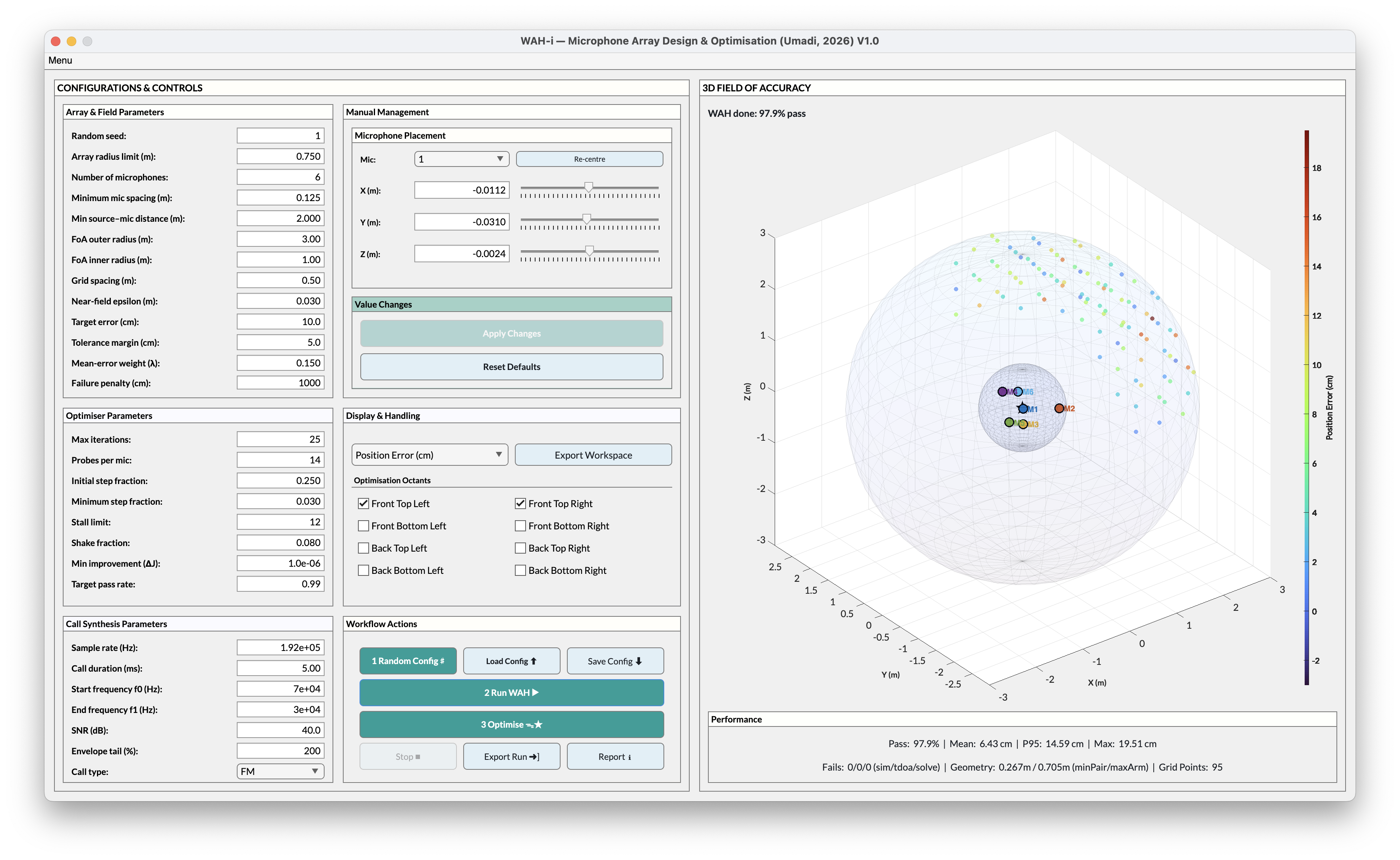
4) Evaluate the baseline geometry

Click Run WAH ▶︎. Apply the Widefield Acoustics Heuristics algorithm to estimate the spatial accuracy at given grid points. (Read the paper)

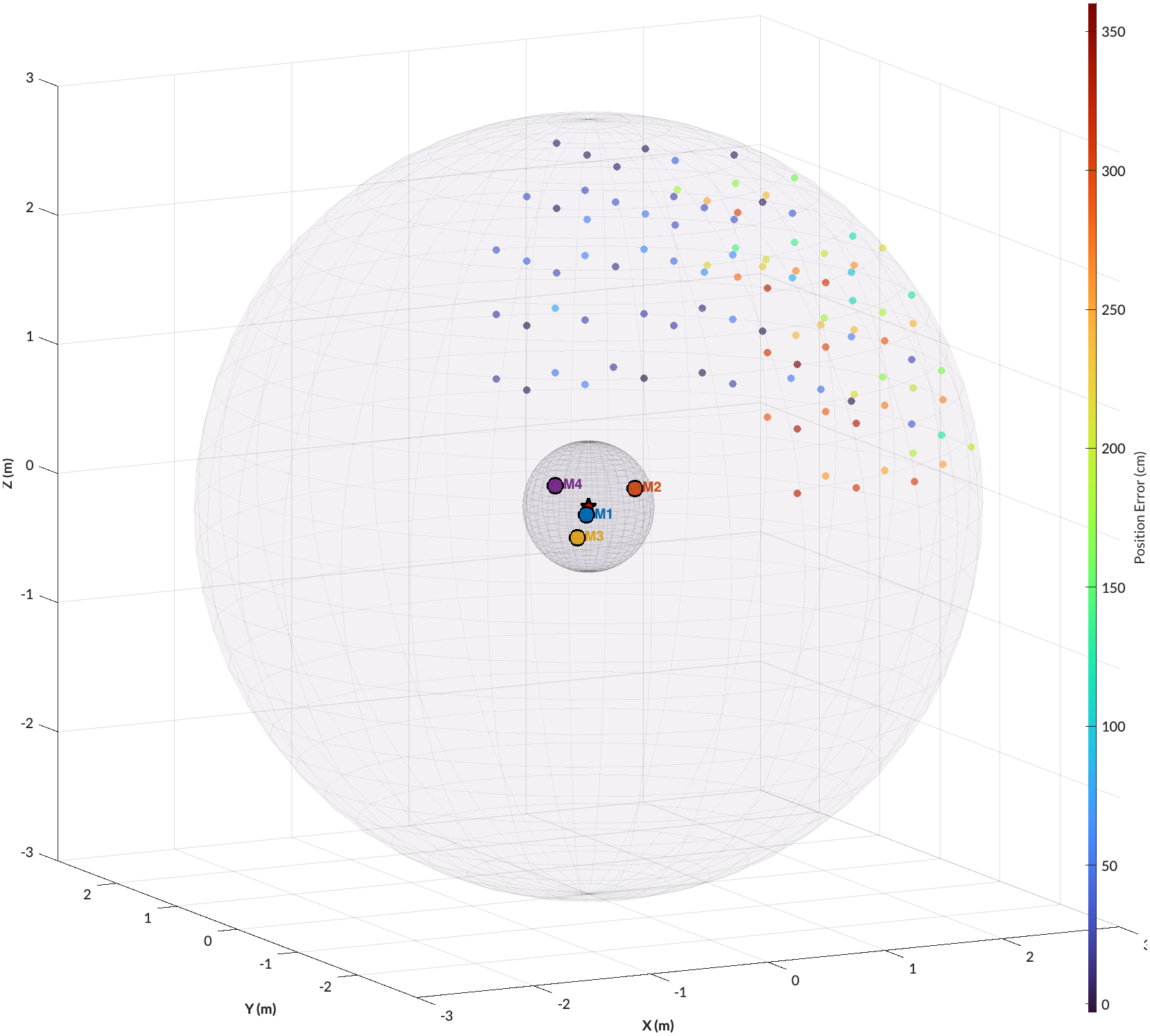
WAH-i evaluates localisation performance across the FoA and displays:

3D colour-coded accuracy field
Summary metrics: Pass rate, Mean, P95, Max error

This baseline evaluation provides a reference for judging optimisation gains.

5) Optimise the geometry

Click Optimise ᯓ★.

For best results:

Start with coarse grid resolution. Increasing grid resolution adds computational costs.
Use conservative step sizes
Increase accuracy thresholds gradually

See Optimisation tips for detailed guidance on staged optimisation strategies.

Example optimisation run showing pass-rate progression and geometry updates — **A successful optimisation run:** A 99% threshold was set for this 6 mic random config at a maximum arm length of 75cm and the optimisation ran with 25 iterations. The front-top octant pairs were restricted to a 1m shell with the FoA set to 3m. The first run with a 50cm arm length achieved about 72% pass rate, which when passed with increased arm length, reached 98% pass rate. Such stagewise optimisation is an ideal approach to explore the best geometries. See the report below.

⬇ Download example high-performance microphone geometry (CSV) (output from the above run)

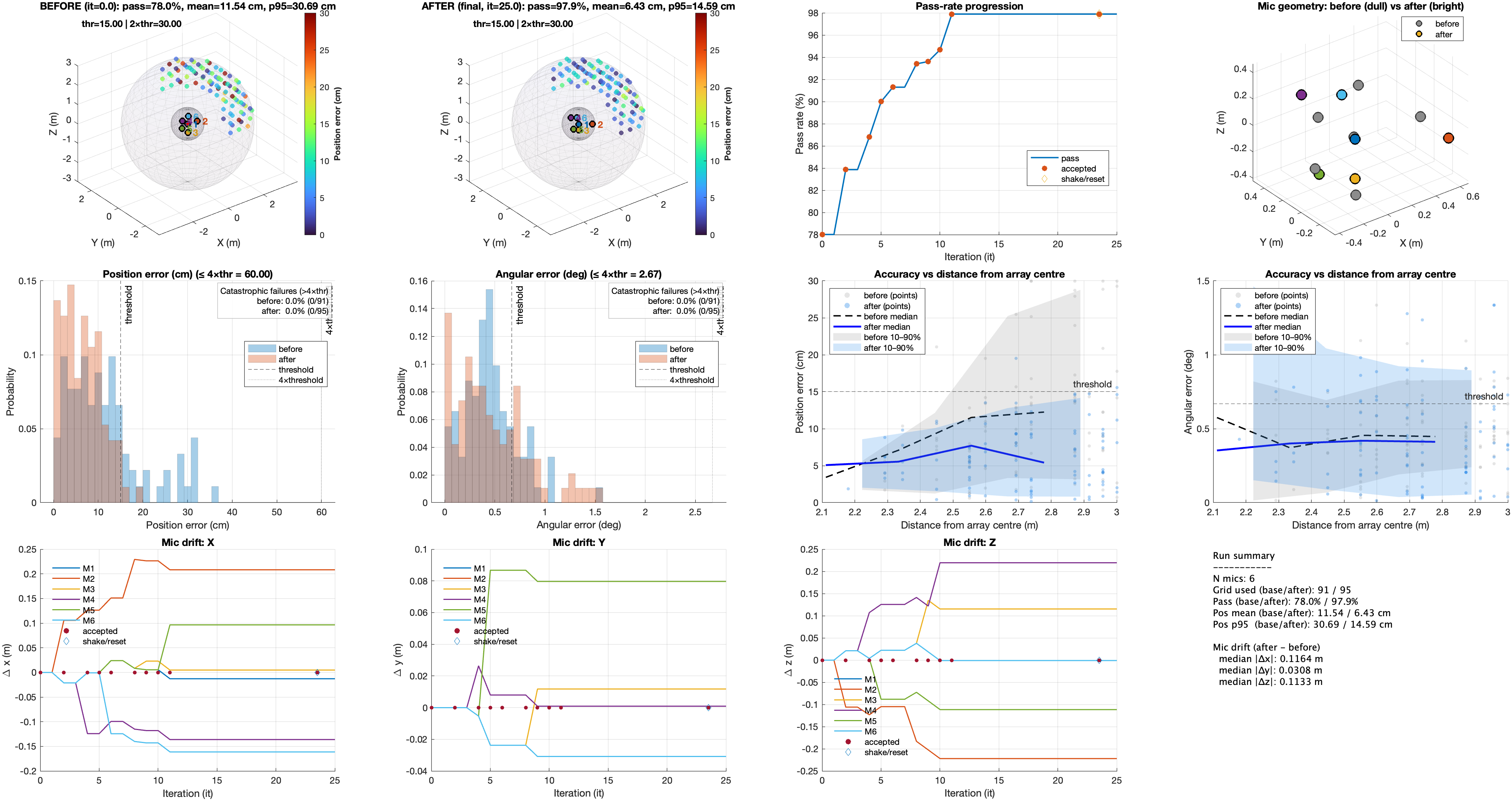
6) Review, export, and save

After optimisation:

View the report to inspect improvements and convergence
Save the report for documentation or sharing
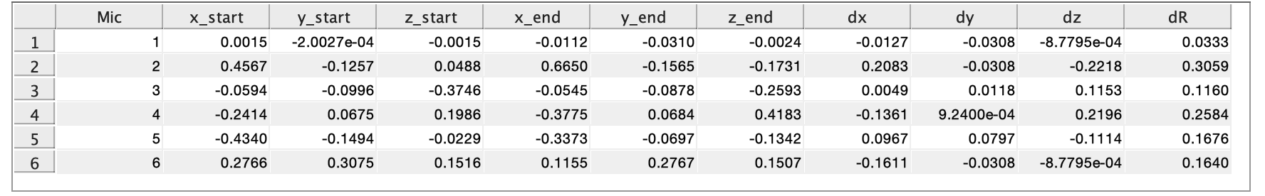
Export .mat file for deeper analysis in MATLAB or Python
Save Config to retain the optimised microphone geometry for future designs

Example optimisation report showing before-and-after performance summaries — **An Example Optimisation report:** Summary of performance improvements, geometry evolution, and spatial accuracy distributions before and after optimisation.

Example optimisation report showing before-and-after mic geometries — **Geometry Summary** The report also produces a summary of the microphones' inital and final geometry, with dimension-wise drift.

This workflow supports rapid iteration while maintaining full reproducibility.

Advanced workflows — batch runs and analyses

For large-scale comparisons or paper-level analyses:

The repository folder mat/ contains batch-run and analysis scripts
These scripts reproduce the full analysis pipeline used in the research paper (see linked publication)

Batch workflows enable:

Comparison of multiple geometries
Repeated optimisation runs
Statistical analysis of convergence and robustness

This is a more advanced workflow and benefits from substantial computational resources.

Design philosophy

WAH-i is intentionally designed so that single-geometry GUI runs are sufficient for most field researchers. Batch analyses are provided for method development, benchmarking, and large comparative studies.